

By Vivek Krishnamoorthy
This submit on Bayesian inference is the second of a multi-part sequence on Bayesian statistics and strategies utilized in quantitative finance.
In my earlier submit, I gave a leisurely introduction to Bayesian statistics and whereas doing so distinguished between the frequentist and the Bayesian outlook of the world. I dwelt on how every of their underlying philosophies influenced their evaluation of assorted probabilistic phenomena. I then mentioned the Bayes’ Theorem together with some illustrations to assist lay the constructing blocks of Bayesian statistics.
Intent of this Put up
My goal right here is to assist develop a deeper understanding of statistical evaluation by specializing in the methodologies adopted by frequentist statistics and Bayesian statistics. I consciously select to deal with the programming and simulation facets utilizing Python in my subsequent submit.
I now instantiate the beforehand mentioned concepts with a easy coin-tossing instance tailored from “Introduction to Bayesian Econometrics (2nd Version)”.
Instance: A Repeated Coin-Tossing Experiment
Suppose we’re taken with estimating the bias of a coin whose equity is unknown. We outline θ (the Greek letter ‘theta’) because the likelihood of getting a head after a coin is tossed. θ is the unknown parameter we need to estimate. We intend to take action by inspecting the outcomes of tossing the coin a number of occasions. Allow us to denote y as a realization of the random variable Y (representing the end result of a coin toss). Let Y=1 if a coin toss ends in heads and Y=0 if a coin toss ends in tails. Primarily, we’re assigning 1 to heads and 0 to tails.
∴ P(Y=1|θ)=θ ; P(Y=0|θ)=1−θ
Primarily based on our above setup, Y will be modelled as a Bernoulli distribution which we denote as
Y ∼ Bernoulli (θ)
I now briefly view our experimental setup by way of the lens of the frequentist and the Bayesian earlier than continuing with our estimation of the unknown parameter θ.
Two Views on the Experiment Setup
In classical statistics (i.e. the frequentist method), our parameter θ is a hard and fast however unknown worth mendacity between 0 and 1. The info we acquire is one realization of a recurrent (i.e. repeating this n-toss experiment say N occasions) experiment. Classical estimation strategies like the strategy of most probability are used to reach at θ̄̂ (known as ‘theta hat’), an estimate for the unknown parameter θ. In statistics, we normally categorical an estimate by placing a hat over the identify of the parameter. I dilate this concept within the subsequent part. To restate what has been mentioned beforehand, we observe that within the frequentist universe, the parameter is mounted however the knowledge is various.
Bayesian statistics is basically totally different. Right here, the parameter θ is handled as a random variable since there’s uncertainty about its worth. It, due to this fact, is sensible for us to treat our parameter as a random variable which could have an related likelihood distribution. So as to apply Bayesian inference, we flip our consideration to one of many elementary legal guidelines of likelihood concept, Bayes’ Theorem that we had seen beforehand.
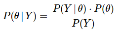
I take advantage of the mathematical type of Bayes’ Theorem as a strategy to set up a reference to Bayesian inference.
……..  (1)
(1)
To repeat what I mentioned in my earlier submit, what makes this theorem so useful is it permits us to invert a conditional likelihood. So if we observe a phenomenon and acquire knowledge or proof about it, the concept helps us analytically outline the conditional likelihood of various potential causes given the proof.
Let’s now apply this to our instance by utilizing the notations we had outlined earlier. I label A = θ and B = y. Within the area of Bayesian statistics, there are particular names used for every of those phrases which I spell out beneath and use subsequently. (1) will be rewritten as:
 …….. (2)
the place:
P(θ) is the prior likelihood. We categorical our perception in regards to the trigger θ BEFORE observing the proof Y. In our instance, the prior can be quantifying our a priori perception on the equity of the coin (right here we will begin with the idea that it’s an unbiased coin, so θ = 1/2). P(Y|θ) is the probability. Right here is the place the actual motion occurs. That is the likelihood of the noticed pattern or proof given the hypothesized trigger. Allow us to, with out lack of generality, assume that we receive 5 heads in 8 coin tosses. Presuming the coin to be unbiased as specified above, the probability can be the likelihood of observing 5 heads in 8 tosses on condition that θ = 1/2. P(θ|Y) is the posterior likelihood. That is the likelihood of the underlying trigger θ AFTER observing the proof y. Right here, we compute our up to date or a posteriori perception on the bias of the coin after observing 5 heads in 8 coin tosses utilizing Bayes’ theorem. P(Y) is the likelihood of the information or proof. We generally additionally name this the marginal probability. That is obtained by taking the weighted sum (or integral) of the probability operate of the proof throughout all potential values of θ. In our instance, we’d compute the likelihood of 5 heads in 8 coin tosses for all potential beliefs about θ. This time period is used to normalize the posterior likelihood. Since it’s unbiased of the parameter to be estimated θ, it’s mathematically extra tractable to precise the posterior likelihood as:
P(θ|Y) ∝ P(Y|θ) × P(θ) …….(3)
(3) is crucial expression in Bayesian statistics and bears repeating. For readability, I paraphrase what I mentioned earlier. Bayesian inference permits us to turnaround conditional possibilities i.e. use the prior possibilities and the probability capabilities to supply a connecting hyperlink to the posterior possibilities i.e. P(θ|Y) granted that we solely know P(Y|θ) and the prior, P(θ). I discover it useful to view (3) as:
Posterior Likelihood ∝ Probability × Prior Likelihood ………. (4)
The experimental goal is to get an estimate of the unknown parameter θ primarily based on the end result of n unbiased coin tosses. The coin tosses generate the pattern or knowledge y = (y1, y2, …, yn), the place yi is 1 or 0 primarily based on the results of the ith coin toss.
I now present the frequentist and Bayesian approaches to fulfilling this goal. Be happy to cursorily skim by way of the derivations I contact upon right here in case you are not within the arithmetic behind it. You possibly can nonetheless develop ample intuitions and be taught to make use of Bayesian strategies in follow.
Estimating θ: The Frequentist Strategy
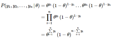
We compute the joint likelihood operate utilizing the utmost probability estimation (MLE) method. The likelihood of the end result for a single coin toss will be elegantly expressed as:
![]()
For a given worth of θ, the joint likelihood of the end result for n unbiased coin tosses is the product of the likelihood of every particular person end result:
 ……. (5)
As we will see in (4), the expression labored out is a operate of the unknown parameter θ given the observations from our experiment. This operate of θ is known as the probability operate and is normally referred to within the literature as:
![]() ……….. (6)
……….. (6)
OR
![]() …………… (7)
…………… (7)
We wish to compute the worth of θ which is more than likely to have yielded the noticed set of outcomes. That is known as the utmost probability estimate, θ̄̂ (‘theta hat’). For analytically computing it, we trivially take the primary order by-product of (6) with respect to the parameter and set it equal to zero. It’s prudent to additionally take the second by-product and examine the signal of its worth at θ = θ̄̂ to make sure that the estimate is certainly the maxima. We frequently typically take the log of the probability operate because it tremendously simplifies the dedication of the utmost probability estimator θ̄̂ . It ought to due to this fact not shock you that the literature is replete with log probability capabilities and their options.
Estimating θ: The Bayesian Strategy
I now change the notations we’ve used to date to make them a bit of extra exact mathematically. I’ll use these notations all through this sequence now. The explanation for this alteration is in order that we will suitably ascribe every time period with symbols that remind us of their random nature. There may be uncertainty over the values of θ, Y, and so on., we, due to this fact, regard them as random variables and assign them corresponding likelihood distributions which I do beneath.
Notations for the Density and Distribution Features
π(⋅) (the Greek letter ‘pi’) to indicate the likelihood distribution operate of the prior (that is pertaining to θ) and π(⋅|y) to indicate the posterior density operate of the parameter we try and estimate.f(⋅) to indicate the likelihood density operate (pdf) for steady random variables and p(.) which is the likelihood mass operate (pmf) of discrete random variables. Nonetheless, for simplicity, I take advantage of f(⋅) regardless of whether or not the random variable Y is steady or discrete.The joint density operate will proceed to be denoted as L(θ|⋅). to indicate the probability operate which is the joint density of the pattern values and is normally the product of the pdf’s/pmf’s of the pattern values from our knowledge.
Do not forget that θ is the parameter we try to estimate.
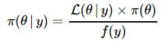
(2) and (3) will be rewritten as
π(θ|y) = [f(y|θ)⋅π(θ)] / f(y) ……(8)
π(θ|y)∝f(y|θ)×π(θ) …………….(9)
Said in phrases, the posterior distribution operate is proportional to the probability operate occasions the prior distribution operate. I redraw your consideration to (4) and current it in congruence with our new notations.
Posterior PDF ∝ Probability × Prior PDF ……….(10)
I now rewrite (8) and (9) utilizing the probability operate L(θ|Y) outlined earlier in (7).
 ……… (11)
![]() ………..(12)
………..(12)
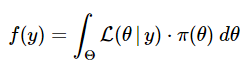
The denominator of (11) is the likelihood distribution of the proof or knowledge. I reiterate what I’ve beforehand talked about whereas inspecting (3): A helpful method of contemplating the posterior density is utilizing the proportionality method as seen in (12). That method, we need not fear in regards to the f(y) time period on the RHS of (11).
For the mathematically curious amongst you, I now take you briefly down a pointless rabbit gap to clarify it incompletely. Maybe, later in our journey, I could write a separate submit brooding on these trivia.
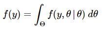
In (11), f(y) is the proportionality fixed that makes the posterior distribution a correct density operate integrating to 1. After we look at it extra carefully, we see that’s, the truth is, the unconditional (marginal) distribution of the random variable Y. We are able to decide it analytically by integrating over all potential values of the parameter θ. Since we’re integrating out θ, we discover that f(y) doesn’t rely on θ.
OR
(11) and (12) signify the continual variations of the Bayes’ Theorem.
The posterior distribution is central to Bayesian statistics and inference as a result of it blends all of the up to date details about the parameter θ in a single expression. This consists of details about θ earlier than the observations have been inspected and that is captured by way of the prior distribution. The knowledge contained within the observations is captured by way of the probability operate.
We are able to regard (11) as a technique of updating info and this concept is additional exemplified by the prior-posterior nomenclature.
The prior distribution of θ, π(θ) represents the data obtainable about its potential values earlier than recording the observations y.The probability operate L(θ|y) of θ is then decided primarily based on the observations y.The posterior distribution of θ, π(θ|y) summarizes all of the obtainable details about the unknown parameter θ after recording and incorporating the observations y.
The Bayesian estimate of θ can be the weighted common of the prior estimate and the utmost probability estimate, θ̄̂ . Because the variety of observations n will increase and approached infinity, the burden on the prior estimate approaches zero and the burden on the MLE approaches one. This means that the Bayesian and frequentist estimates would converge as our pattern measurement will get bigger.
To make clear, in a classical or frequentist setting, the standard estimator of the parameter, θ is the ML estimator, θ̄̂ . Right here, the prior is implicitly handled as a continuing.
Abstract
I’ve devoted this submit to deriving the elemental results of Bayesian statistics, viz. (10) . The essence of this expression is to signify uncertainty by combining the information obtained from two sources – observations and prior beliefs. In doing so, I launched the ideas of prior distributions, probability capabilities and posterior distributions in addition to the comparability of the frequentist and Bayesian methodologies. In my subsequent submit, I intend to make good my promise of illustrating the above instance with simulations in Python.
Bayesian statistics is a crucial a part of quantitative methods that are a part of an algorithmic dealer’s handbook. The Government Programme in Algorithmic Buying and selling (EPAT™) course by QuantInsti® covers coaching modules like Statistics & Econometrics, Monetary Computing & Know-how, and Algorithmic & Quantitative Buying and selling that equip you with the required talent units for making use of varied buying and selling devices and platforms to be a profitable dealer.
Disclaimer: All investments and buying and selling within the inventory market contain threat. Any selections to position trades within the monetary markets, together with buying and selling in inventory or choices or different monetary devices is a private resolution that ought to solely be made after thorough analysis, together with a private threat and monetary evaluation and the engagement {of professional} help to the extent you imagine obligatory. The buying and selling methods or associated info talked about on this article is for informational functions solely.


